Download A Datatable On R
Get source code for this RMarkdown script here.
Consider being a patron and supporting my work?
Donate and become a patron: If you find value in what I do and have learned something from my site, please consider becoming a patron. It takes me many hours to research, learn, and put together tutorials. Your support really matters.
Load packages/libraries
Use library() to load packages at the top of each R script.
library(data.table); library(tidyverse) library(hausekeep) # if you don't have my package and want to use it, you'll have to install it from github # devtools::install_github("hauselin/hausekeep") # you might have to install devtools first (see above) Reading data into R
Read file in a directory and save the data as an object in the environment by using the assignment <- operator. `
If you don't have the dataset, right click here to download and save sleep.csv dataset. If you're following the tutorial step by step, you should also create a data folder in your current folder, and put the sleep.csv file inside the data folder.
df1 <- read.csv("./data/sleep.csv") # base R read.csv() function # same as df1 <- read.csv("data/sleep.csv") # READ: assign the output return by read.csv("data/sleep.csv") into df1 df2 <- fread("./data/sleep.csv") # fread() from library(data.table) # my favorite is fread from data.table df3 <- fread("data/sleep.csv") # same as above # or download data from website directly url <- "https://raw.githubusercontent.com/hauselin/rtutorialsite/master/data/sleep.csv" df_url <- fread(url) I always use fread() from the data.table to read data now. It's super intelligent and fast (reads gigabytes of data in just a few seconds).
The . in the file path simply refers to the current working directory, so it can be dropped. And .. can be used to refer to the parent directory. If your current directory is /home/desktop, then . refers to just that, and .. refers to the parent directory of your current directory, which is the /home directory.
Comparing the outputs of read.csv(x) and fread(x)
df1 # output of read.csv("./data/sleep.csv") extra group ID 1 0.7 1 1 2 -1.6 1 2 3 -0.2 1 3 4 -1.2 1 4 5 -0.1 1 5 6 3.4 1 6 7 3.7 1 7 8 0.8 1 8 9 0.0 1 9 10 2.0 1 10 11 1.9 2 1 12 0.8 2 2 13 1.1 2 3 14 0.1 2 4 15 -0.1 2 5 16 4.4 2 6 17 5.5 2 7 18 1.6 2 8 19 4.6 2 9 20 3.4 2 10 class(df1) # read.csv("./data/sleep.csv") [1] "data.frame" How's the output different from the one above?
df3 # output of fread("./data/sleep.csv") extra group ID 1: 0.7 1 1 2: -1.6 1 2 3: -0.2 1 3 4: -1.2 1 4 5: -0.1 1 5 6: 3.4 1 6 7: 3.7 1 7 8: 0.8 1 8 9: 0.0 1 9 10: 2.0 1 10 11: 1.9 2 1 12: 0.8 2 2 13: 1.1 2 3 14: 0.1 2 4 15: -0.1 2 5 16: 4.4 2 6 17: 5.5 2 7 18: 1.6 2 8 19: 4.6 2 9 20: 3.4 2 10 class(df3) # fread("./data/sleep.csv") [1] "data.table" "data.frame" How's the output different from the two outputs above?
Reading URLs and other formats
Check out the csv (comma separated values) data here. You can read data directly off a website.
Most of these read functions can import/read different types of files (e.g., csv, txt, URLs) as long as the raw data are formatted properly (e.g., separated by commas, tabs). But if you're trying to read proprietary data formats (e.g., SPSS datasets, Excel sheets), you'll need to use other libraries (e.g., readxl, foreign) to read those data into R.
df_url <- fread("https://raw.githubusercontent.com/hauselin/rtutorialsite/master/data/sleep.csv") df_url # print data to console; same dataset fread("data/sleep.csv") extra group ID 1: 0.7 1 1 2: -1.6 1 2 3: -0.2 1 3 4: -1.2 1 4 5: -0.1 1 5 6: 3.4 1 6 7: 3.7 1 7 8: 0.8 1 8 9: 0.0 1 9 10: 2.0 1 10 11: 1.9 2 1 12: 0.8 2 2 13: 1.1 2 3 14: 0.1 2 4 15: -0.1 2 5 16: 4.4 2 6 17: 5.5 2 7 18: 1.6 2 8 19: 4.6 2 9 20: 3.4 2 10 Summarizing objects
You can summarize objects quickly by using summary(), str(), glimpse(), or print(x, n).
To view the first/last few items of an object, use head() or tail().
df3 # see entire data.table extra group ID 1: 0.7 1 1 2: -1.6 1 2 3: -0.2 1 3 4: -1.2 1 4 5: -0.1 1 5 6: 3.4 1 6 7: 3.7 1 7 8: 0.8 1 8 9: 0.0 1 9 10: 2.0 1 10 11: 1.9 2 1 12: 0.8 2 2 13: 1.1 2 3 14: 0.1 2 4 15: -0.1 2 5 16: 4.4 2 6 17: 5.5 2 7 18: 1.6 2 8 19: 4.6 2 9 20: 3.4 2 10 summary(df3) # we use summary() for many many other purposes extra group ID Min. :-1.600 Min. :1.0 Min. : 1.0 1st Qu.:-0.025 1st Qu.:1.0 1st Qu.: 3.0 Median : 0.950 Median :1.5 Median : 5.5 Mean : 1.540 Mean :1.5 Mean : 5.5 3rd Qu.: 3.400 3rd Qu.:2.0 3rd Qu.: 8.0 Max. : 5.500 Max. :2.0 Max. :10.0 str(df3) Classes 'data.table' and 'data.frame': 20 obs. of 3 variables: $ extra: num 0.7 -1.6 -0.2 -1.2 -0.1 3.4 3.7 0.8 0 2 ... $ group: int 1 1 1 1 1 1 1 1 1 1 ... $ ID : int 1 2 3 4 5 6 7 8 9 10 ... - attr(*, ".internal.selfref")=<externalptr> glimpse(df3) Rows: 20 Columns: 3 $ extra <dbl> 0.7, -1.6, -0.2, -1.2, -0.1, 3.4, 3.7, 0.8, 0.0, 2.0, 1.9, 0.8,… $ group <int> 1, 1, 1, 1, 1, 1, 1, 1, 1, 1, 2, 2, 2, 2, 2, 2, 2, 2, 2, 2 $ ID <int> 1, 2, 3, 4, 5, 6, 7, 8, 9, 10, 1, 2, 3, 4, 5, 6, 7, 8, 9, 10 head(df3) extra group ID 1: 0.7 1 1 2: -1.6 1 2 3: -0.2 1 3 4: -1.2 1 4 5: -0.1 1 5 6: 3.4 1 6 head(df3, n = 3) # what does this do? extra group ID 1: 0.7 1 1 2: -1.6 1 2 3: -0.2 1 3 tail(df3, n = 2) extra group ID 1: 4.6 2 9 2: 3.4 2 10 dim(df3) # dimensions (row by columns) [1] 20 3 Use pipes %>% to summarize objects
df3 %>% head(n = 2) extra group ID 1: 0.7 1 1 2: -1.6 1 2 df3 %>% head(2) # why does this work? extra group ID 1: 0.7 1 1 2: -1.6 1 2 df3 %>% summary() # does this work? why? extra group ID Min. :-1.600 Min. :1.0 Min. : 1.0 1st Qu.:-0.025 1st Qu.:1.0 1st Qu.: 3.0 Median : 0.950 Median :1.5 Median : 5.5 Mean : 1.540 Mean :1.5 Mean : 5.5 3rd Qu.: 3.400 3rd Qu.:2.0 3rd Qu.: 8.0 Max. : 5.500 Max. :2.0 Max. :10.0 Using $ and [] to extract elements using their names
names(df3) [1] "extra" "group" "ID" df3$extra # extracts column/variable as a vector [1] 0.7 -1.6 -0.2 -1.2 -0.1 3.4 3.7 0.8 0.0 2.0 1.9 0.8 1.1 0.1 -0.1 [16] 4.4 5.5 1.6 4.6 3.4 df3$group [1] 1 1 1 1 1 1 1 1 1 1 2 2 2 2 2 2 2 2 2 2 df3$ID [1] 1 2 3 4 5 6 7 8 9 10 1 2 3 4 5 6 7 8 9 10 # create a list with named items a, b, c myList <- list(a = -999, b = c(TRUE, FALSE, T, T), c = c('my_amazing_list')) class(myList) [1] "list" names(myList) [1] "a" "b" "c" myList # note the structure of a list ($ signs tell you how to get items) $a [1] -999 $b [1] TRUE FALSE TRUE TRUE $c [1] "my_amazing_list" myList$a [1] -999 myList$b [1] TRUE FALSE TRUE TRUE myList$c [1] "my_amazing_list" # same as df1$extra, but use characters (in '') to extract elements df1['extra'] extra 1 0.7 2 -1.6 3 -0.2 4 -1.2 5 -0.1 6 3.4 7 3.7 8 0.8 9 0.0 10 2.0 11 1.9 12 0.8 13 1.1 14 0.1 15 -0.1 16 4.4 17 5.5 18 1.6 19 4.6 20 3.4 ** BUT the syntax above only works for the data.frame class!**
df3['extra'] # fails!!! Error in `[.data.table`(df3, "extra"): When i is a data.table (or character vector), the columns to join by must be specified using 'on=' argument (see ?data.table), by keying x (i.e. sorted, and, marked as sorted, see ?setkey), or by sharing column names between x and i (i.e., a natural join). Keyed joins might have further speed benefits on very large data due to x being sorted in RAM. If it's a data.table class, you do it differently (so know the classes of your objects)! But more on data.table later on.
df3[, 'extra'] # df3[i, j] (i is row, and j is column) extra 1: 0.7 2: -1.6 3: -0.2 4: -1.2 5: -0.1 6: 3.4 7: 3.7 8: 0.8 9: 0.0 10: 2.0 11: 1.9 12: 0.8 13: 1.1 14: 0.1 15: -0.1 16: 4.4 17: 5.5 18: 1.6 19: 4.6 20: 3.4 # df3$extra also works for data.table Writing/saving dataframes or datatables as csv files
IMPORTANT: The functions below overwrite any existing files that have the same name and you can't recover the original file if you've overwritten it!
# save data to your working directory # data.table's fwrite fwrite(df3, 'example1_df3.csv') # save data to the data inside your current directory, assuming it exists! fwrite(df3, 'data/example1_df3.csv') The more common base R function is write.csv() but I never use it now and always use fwrite from data.table, which works for any type of dataframe you want to save (not limited to data.table).
Here's the base R function. Note that you'll have to specify row.names = F to prevent write.csv() from adding an extra column with row numbers when it saves the data (another reason to use fwrite instead).
# saves in your working directory write.csv(df3, 'example1_df3.csv', row.names = F) # saves in your data directory (assumes data directory exists!) write.csv(df3, './data/example2_df3.csv', row.names = F) tidyverse: a collection of R packages
tidyverse:
The tidyverse is an opinionated collection of R packages designed for data science. All packages share an underlying design philosophy, grammar, and data structures.
Included packages: ggplot2, dplyr, tidyr, stringr etc. see official website for documentation
I'm running library(tidyverse) here for educational purposes; you only need to load packages once per R session you're running (we already loaded our packages at the top of this script).
Manipulating datasets with dplyr (a package in tidyverse)
Read in data from a csv file (stored in "./data/simpsonsParadox.csv"). Right-click to download and save the data here (you can also use the fread() function to read and download it directly from the URL; see code below)
-
fread(): a function fromdata.table(fast-read, hence fread) that is VERY fast and powerful, and much better thanread.csv()orread.table()from base R
df4 <- fread("./data/simpsonsParadox.csv") # or download data directly from URL url <- "https://raw.githubusercontent.com/hauselin/rtutorialsite/master/data/simpsonsParadox.csv" df4 <- fread(url) class(df4) # note it's a data.table AND a data.frame [1] "data.table" "data.frame" dim(df4) # no. of rows and columns [1] 40 3 glimpse(df4) # have a glimpse of the data (quick summary of data and column classes) Rows: 40 Columns: 3 $ iq <dbl> 94.5128, 95.4359, 97.7949, 98.1026, 96.5641, 101.5897, 100.871… $ grades <dbl> 67.9295, 82.5449, 69.0833, 83.3141, 99.0833, 89.8526, 73.6987,… $ class <chr> "a", "a", "a", "a", "a", "a", "a", "a", "a", "a", "b", "b", "b… # str(df4) # similar to glimpse glimpse() summarizes your data and tells you how many rows/columns you have and the class of each column.
-
dbl: double (a type of number with decimal places) -
chr: character/string
Select columns/variables with select()
Select with names
select(df4, iq) # just prints the output to console without saving iq 1: 94.5128 2: 95.4359 3: 97.7949 4: 98.1026 5: 96.5641 6: 101.5897 7: 100.8718 8: 97.0769 9: 94.2051 10: 94.4103 11: 103.7436 12: 102.8205 13: 101.5897 14: 105.3846 15: 106.4103 16: 109.4872 17: 107.2308 18: 107.2308 19: 102.1026 20: 100.0513 21: 111.0256 22: 114.7179 23: 112.2564 24: 108.6667 25: 110.5128 26: 114.1026 27: 115.0256 28: 118.7179 29: 112.8718 30: 118.0000 31: 116.9744 32: 121.1795 33: 117.6923 34: 121.8974 35: 123.6410 36: 121.3846 37: 123.7436 38: 124.7692 39: 124.8718 40: 127.6410 iq df4_iq <- select(df4, iq) # if you want to save as a new object df4_iq # print df4_iq iq 1: 94.5128 2: 95.4359 3: 97.7949 4: 98.1026 5: 96.5641 6: 101.5897 7: 100.8718 8: 97.0769 9: 94.2051 10: 94.4103 11: 103.7436 12: 102.8205 13: 101.5897 14: 105.3846 15: 106.4103 16: 109.4872 17: 107.2308 18: 107.2308 19: 102.1026 20: 100.0513 21: 111.0256 22: 114.7179 23: 112.2564 24: 108.6667 25: 110.5128 26: 114.1026 27: 115.0256 28: 118.7179 29: 112.8718 30: 118.0000 31: 116.9744 32: 121.1795 33: 117.6923 34: 121.8974 35: 123.6410 36: 121.3846 37: 123.7436 38: 124.7692 39: 124.8718 40: 127.6410 iq # select without assigning/saving output to a variable/object select(df4, class, grades) class grades 1: a 67.9295 2: a 82.5449 3: a 69.0833 4: a 83.3141 5: a 99.0833 6: a 89.8526 7: a 73.6987 8: a 47.9295 9: a 55.6218 10: a 44.4679 11: b 74.0833 12: b 59.8526 13: b 47.9295 14: b 44.8526 15: b 60.2372 16: b 64.8526 17: b 74.4679 18: b 49.8526 19: b 37.9295 20: b 54.8526 21: c 56.0064 22: c 56.0064 23: c 46.3910 24: c 43.6987 25: c 36.3910 26: c 30.2372 27: c 39.4679 28: c 51.0064 29: c 64.0833 30: c 55.3000 31: d 17.5449 32: d 35.2372 33: d 29.8526 34: d 18.3141 35: d 29.4679 36: d 53.6987 37: d 63.6987 38: d 48.6987 39: d 38.3141 40: d 51.7756 class grades select(df4, iq, grades) iq grades 1: 94.5128 67.9295 2: 95.4359 82.5449 3: 97.7949 69.0833 4: 98.1026 83.3141 5: 96.5641 99.0833 6: 101.5897 89.8526 7: 100.8718 73.6987 8: 97.0769 47.9295 9: 94.2051 55.6218 10: 94.4103 44.4679 11: 103.7436 74.0833 12: 102.8205 59.8526 13: 101.5897 47.9295 14: 105.3846 44.8526 15: 106.4103 60.2372 16: 109.4872 64.8526 17: 107.2308 74.4679 18: 107.2308 49.8526 19: 102.1026 37.9295 20: 100.0513 54.8526 21: 111.0256 56.0064 22: 114.7179 56.0064 23: 112.2564 46.3910 24: 108.6667 43.6987 25: 110.5128 36.3910 26: 114.1026 30.2372 27: 115.0256 39.4679 28: 118.7179 51.0064 29: 112.8718 64.0833 30: 118.0000 55.3000 31: 116.9744 17.5449 32: 121.1795 35.2372 33: 117.6923 29.8526 34: 121.8974 18.3141 35: 123.6410 29.4679 36: 121.3846 53.6987 37: 123.7436 63.6987 38: 124.7692 48.6987 39: 124.8718 38.3141 40: 127.6410 51.7756 iq grades Select multiple columns in sequence with :
select(df4, iq:class) iq grades class 1: 94.5128 67.9295 a 2: 95.4359 82.5449 a 3: 97.7949 69.0833 a 4: 98.1026 83.3141 a 5: 96.5641 99.0833 a 6: 101.5897 89.8526 a 7: 100.8718 73.6987 a 8: 97.0769 47.9295 a 9: 94.2051 55.6218 a 10: 94.4103 44.4679 a 11: 103.7436 74.0833 b 12: 102.8205 59.8526 b 13: 101.5897 47.9295 b 14: 105.3846 44.8526 b 15: 106.4103 60.2372 b 16: 109.4872 64.8526 b 17: 107.2308 74.4679 b 18: 107.2308 49.8526 b 19: 102.1026 37.9295 b 20: 100.0513 54.8526 b 21: 111.0256 56.0064 c 22: 114.7179 56.0064 c 23: 112.2564 46.3910 c 24: 108.6667 43.6987 c 25: 110.5128 36.3910 c 26: 114.1026 30.2372 c 27: 115.0256 39.4679 c 28: 118.7179 51.0064 c 29: 112.8718 64.0833 c 30: 118.0000 55.3000 c 31: 116.9744 17.5449 d 32: 121.1795 35.2372 d 33: 117.6923 29.8526 d 34: 121.8974 18.3141 d 35: 123.6410 29.4679 d 36: 121.3846 53.6987 d 37: 123.7436 63.6987 d 38: 124.7692 48.6987 d 39: 124.8718 38.3141 d 40: 127.6410 51.7756 d iq grades class Select with numbers
select(df4, 1, 3) iq class 1: 94.5128 a 2: 95.4359 a 3: 97.7949 a 4: 98.1026 a 5: 96.5641 a 6: 101.5897 a 7: 100.8718 a 8: 97.0769 a 9: 94.2051 a 10: 94.4103 a 11: 103.7436 b 12: 102.8205 b 13: 101.5897 b 14: 105.3846 b 15: 106.4103 b 16: 109.4872 b 17: 107.2308 b 18: 107.2308 b 19: 102.1026 b 20: 100.0513 b 21: 111.0256 c 22: 114.7179 c 23: 112.2564 c 24: 108.6667 c 25: 110.5128 c 26: 114.1026 c 27: 115.0256 c 28: 118.7179 c 29: 112.8718 c 30: 118.0000 c 31: 116.9744 d 32: 121.1795 d 33: 117.6923 d 34: 121.8974 d 35: 123.6410 d 36: 121.3846 d 37: 123.7436 d 38: 124.7692 d 39: 124.8718 d 40: 127.6410 d iq class select(df4, 1:3) # what does 1:3 do? run 1:3 in your console iq grades class 1: 94.5128 67.9295 a 2: 95.4359 82.5449 a 3: 97.7949 69.0833 a 4: 98.1026 83.3141 a 5: 96.5641 99.0833 a 6: 101.5897 89.8526 a 7: 100.8718 73.6987 a 8: 97.0769 47.9295 a 9: 94.2051 55.6218 a 10: 94.4103 44.4679 a 11: 103.7436 74.0833 b 12: 102.8205 59.8526 b 13: 101.5897 47.9295 b 14: 105.3846 44.8526 b 15: 106.4103 60.2372 b 16: 109.4872 64.8526 b 17: 107.2308 74.4679 b 18: 107.2308 49.8526 b 19: 102.1026 37.9295 b 20: 100.0513 54.8526 b 21: 111.0256 56.0064 c 22: 114.7179 56.0064 c 23: 112.2564 46.3910 c 24: 108.6667 43.6987 c 25: 110.5128 36.3910 c 26: 114.1026 30.2372 c 27: 115.0256 39.4679 c 28: 118.7179 51.0064 c 29: 112.8718 64.0833 c 30: 118.0000 55.3000 c 31: 116.9744 17.5449 d 32: 121.1795 35.2372 d 33: 117.6923 29.8526 d 34: 121.8974 18.3141 d 35: 123.6410 29.4679 d 36: 121.3846 53.6987 d 37: 123.7436 63.6987 d 38: 124.7692 48.6987 d 39: 124.8718 38.3141 d 40: 127.6410 51.7756 d iq grades class How can we reorder columns with select()?
select(df4, 3:1) # column 3, then 2, then 1 class grades iq 1: a 67.9295 94.5128 2: a 82.5449 95.4359 3: a 69.0833 97.7949 4: a 83.3141 98.1026 5: a 99.0833 96.5641 6: a 89.8526 101.5897 7: a 73.6987 100.8718 8: a 47.9295 97.0769 9: a 55.6218 94.2051 10: a 44.4679 94.4103 11: b 74.0833 103.7436 12: b 59.8526 102.8205 13: b 47.9295 101.5897 14: b 44.8526 105.3846 15: b 60.2372 106.4103 16: b 64.8526 109.4872 17: b 74.4679 107.2308 18: b 49.8526 107.2308 19: b 37.9295 102.1026 20: b 54.8526 100.0513 21: c 56.0064 111.0256 22: c 56.0064 114.7179 23: c 46.3910 112.2564 24: c 43.6987 108.6667 25: c 36.3910 110.5128 26: c 30.2372 114.1026 27: c 39.4679 115.0256 28: c 51.0064 118.7179 29: c 64.0833 112.8718 30: c 55.3000 118.0000 31: d 17.5449 116.9744 32: d 35.2372 121.1795 33: d 29.8526 117.6923 34: d 18.3141 121.8974 35: d 29.4679 123.6410 36: d 53.6987 121.3846 37: d 63.6987 123.7436 38: d 48.6987 124.7692 39: d 38.3141 124.8718 40: d 51.7756 127.6410 class grades iq Select with starts_with() or ends_with()
select(df4, starts_with("c")) class 1: a 2: a 3: a 4: a 5: a 6: a 7: a 8: a 9: a 10: a 11: b 12: b 13: b 14: b 15: b 16: b 17: b 18: b 19: b 20: b 21: c 22: c 23: c 24: c 25: c 26: c 27: c 28: c 29: c 30: c 31: d 32: d 33: d 34: d 35: d 36: d 37: d 38: d 39: d 40: d class select(df4, starts_with("g")) grades 1: 67.9295 2: 82.5449 3: 69.0833 4: 83.3141 5: 99.0833 6: 89.8526 7: 73.6987 8: 47.9295 9: 55.6218 10: 44.4679 11: 74.0833 12: 59.8526 13: 47.9295 14: 44.8526 15: 60.2372 16: 64.8526 17: 74.4679 18: 49.8526 19: 37.9295 20: 54.8526 21: 56.0064 22: 56.0064 23: 46.3910 24: 43.6987 25: 36.3910 26: 30.2372 27: 39.4679 28: 51.0064 29: 64.0833 30: 55.3000 31: 17.5449 32: 35.2372 33: 29.8526 34: 18.3141 35: 29.4679 36: 53.6987 37: 63.6987 38: 48.6987 39: 38.3141 40: 51.7756 grades select(df4, starts_with("g"), ends_with("s")) grades class 1: 67.9295 a 2: 82.5449 a 3: 69.0833 a 4: 83.3141 a 5: 99.0833 a 6: 89.8526 a 7: 73.6987 a 8: 47.9295 a 9: 55.6218 a 10: 44.4679 a 11: 74.0833 b 12: 59.8526 b 13: 47.9295 b 14: 44.8526 b 15: 60.2372 b 16: 64.8526 b 17: 74.4679 b 18: 49.8526 b 19: 37.9295 b 20: 54.8526 b 21: 56.0064 c 22: 56.0064 c 23: 46.3910 c 24: 43.6987 c 25: 36.3910 c 26: 30.2372 c 27: 39.4679 c 28: 51.0064 c 29: 64.0833 c 30: 55.3000 c 31: 17.5449 d 32: 35.2372 d 33: 29.8526 d 34: 18.3141 d 35: 29.4679 d 36: 53.6987 d 37: 63.6987 d 38: 48.6987 d 39: 38.3141 d 40: 51.7756 d grades class Dropping columns with -
select(df4, -grades) # what should you get? iq class 1: 94.5128 a 2: 95.4359 a 3: 97.7949 a 4: 98.1026 a 5: 96.5641 a 6: 101.5897 a 7: 100.8718 a 8: 97.0769 a 9: 94.2051 a 10: 94.4103 a 11: 103.7436 b 12: 102.8205 b 13: 101.5897 b 14: 105.3846 b 15: 106.4103 b 16: 109.4872 b 17: 107.2308 b 18: 107.2308 b 19: 102.1026 b 20: 100.0513 b 21: 111.0256 c 22: 114.7179 c 23: 112.2564 c 24: 108.6667 c 25: 110.5128 c 26: 114.1026 c 27: 115.0256 c 28: 118.7179 c 29: 112.8718 c 30: 118.0000 c 31: 116.9744 d 32: 121.1795 d 33: 117.6923 d 34: 121.8974 d 35: 123.6410 d 36: 121.3846 d 37: 123.7436 d 38: 124.7692 d 39: 124.8718 d 40: 127.6410 d iq class select(df4, -ends_with("s")) # what should you get? iq 1: 94.5128 2: 95.4359 3: 97.7949 4: 98.1026 5: 96.5641 6: 101.5897 7: 100.8718 8: 97.0769 9: 94.2051 10: 94.4103 11: 103.7436 12: 102.8205 13: 101.5897 14: 105.3846 15: 106.4103 16: 109.4872 17: 107.2308 18: 107.2308 19: 102.1026 20: 100.0513 21: 111.0256 22: 114.7179 23: 112.2564 24: 108.6667 25: 110.5128 26: 114.1026 27: 115.0256 28: 118.7179 29: 112.8718 30: 118.0000 31: 116.9744 32: 121.1795 33: 117.6923 34: 121.8974 35: 123.6410 36: 121.3846 37: 123.7436 38: 124.7692 39: 124.8718 40: 127.6410 iq select(df4, -ends_with("s"), class, -1) # what should you get? class 1: a 2: a 3: a 4: a 5: a 6: a 7: a 8: a 9: a 10: a 11: b 12: b 13: b 14: b 15: b 16: b 17: b 18: b 19: b 20: b 21: c 22: c 23: c 24: c 25: c 26: c 27: c 28: c 29: c 30: c 31: d 32: d 33: d 34: d 35: d 36: d 37: d 38: d 39: d 40: d class Renaming while selecting columns/variables
select(df4, intelligence = iq) # select iq and rename it to intelligence intelligence 1: 94.5128 2: 95.4359 3: 97.7949 4: 98.1026 5: 96.5641 6: 101.5897 7: 100.8718 8: 97.0769 9: 94.2051 10: 94.4103 11: 103.7436 12: 102.8205 13: 101.5897 14: 105.3846 15: 106.4103 16: 109.4872 17: 107.2308 18: 107.2308 19: 102.1026 20: 100.0513 21: 111.0256 22: 114.7179 23: 112.2564 24: 108.6667 25: 110.5128 26: 114.1026 27: 115.0256 28: 118.7179 29: 112.8718 30: 118.0000 31: 116.9744 32: 121.1795 33: 117.6923 34: 121.8974 35: 123.6410 36: 121.3846 37: 123.7436 38: 124.7692 39: 124.8718 40: 127.6410 intelligence Other options for select() include matches(), contains(). For more information, see tutorial/vignette here. For official documentation, see here.
Select rows with slice()
slice(df4, 1:5) # rows 1 to 5 iq grades class 1: 94.5128 67.9295 a 2: 95.4359 82.5449 a 3: 97.7949 69.0833 a 4: 98.1026 83.3141 a 5: 96.5641 99.0833 a slice(df4, c(1, 3, 5, 7, 9)) # rows 1, 3, 5, 7, 9 iq grades class 1: 94.5128 67.9295 a 2: 97.7949 69.0833 a 3: 96.5641 99.0833 a 4: 100.8718 73.6987 a 5: 94.2051 55.6218 a slice(df4, seq(from = 1, to = 10, by = 2)) # same as above, but using sequence function (from 1 to 10, by/in steps of 2) iq grades class 1: 94.5128 67.9295 a 2: 97.7949 69.0833 a 3: 96.5641 99.0833 a 4: 100.8718 73.6987 a 5: 94.2051 55.6218 a slice(df4, -c(1:39)) # remove rows 1 to 39 iq grades class 1: 127.641 51.7756 d Filtering or subsetting data/rows with filter()
While select() acts on columns, filter() acts on rows. It chooses/subsets rows based on criteria you specify.
How many classes are there in this dataset? How many unique classes?
df4$class [1] "a" "a" "a" "a" "a" "a" "a" "a" "a" "a" "b" "b" "b" "b" "b" "b" "b" "b" "b" [20] "b" "c" "c" "c" "c" "c" "c" "c" "c" "c" "c" "d" "d" "d" "d" "d" "d" "d" "d" [39] "d" "d" unique(df4$class) # unique classes [1] "a" "b" "c" "d" df4$class %>% unique() # same as above but with pipes [1] "a" "b" "c" "d" Filter rows that match one criterion
filter(df4, class == "a") # how many rows of data do we have now? iq grades class 1: 94.5128 67.9295 a 2: 95.4359 82.5449 a 3: 97.7949 69.0833 a 4: 98.1026 83.3141 a 5: 96.5641 99.0833 a 6: 101.5897 89.8526 a 7: 100.8718 73.6987 a 8: 97.0769 47.9295 a 9: 94.2051 55.6218 a 10: 94.4103 44.4679 a filter(df4, class == 'b') # R accepths single or double quotations iq grades class 1: 103.7436 74.0833 b 2: 102.8205 59.8526 b 3: 101.5897 47.9295 b 4: 105.3846 44.8526 b 5: 106.4103 60.2372 b 6: 109.4872 64.8526 b 7: 107.2308 74.4679 b 8: 107.2308 49.8526 b 9: 102.1026 37.9295 b 10: 100.0513 54.8526 b df4_classA <- filter(df4, class == 'a') # to save filtered data as an object df4_classA iq grades class 1: 94.5128 67.9295 a 2: 95.4359 82.5449 a 3: 97.7949 69.0833 a 4: 98.1026 83.3141 a 5: 96.5641 99.0833 a 6: 101.5897 89.8526 a 7: 100.8718 73.6987 a 8: 97.0769 47.9295 a 9: 94.2051 55.6218 a 10: 94.4103 44.4679 a Filter rows that match multiple criteria with %in%
Let's say you want to get the rows where the class variable is a or b. You might write the following:
filter(df4, class == c("a", "b")) What's wrong? Look at the output and compare with filter(df4, class == "a") and filter(df4, class == "b"). How many rows should you expect from filter(df4, class == c("a", "b"))? How many rows did you get?
Here's how to do it correctly. You use %in% if you want to match multiple criteria. == only works if you're matching by just ONE criterion
filter(df4, class %in% c("a", "b")) # check number of rows of output iq grades class 1: 94.5128 67.9295 a 2: 95.4359 82.5449 a 3: 97.7949 69.0833 a 4: 98.1026 83.3141 a 5: 96.5641 99.0833 a 6: 101.5897 89.8526 a 7: 100.8718 73.6987 a 8: 97.0769 47.9295 a 9: 94.2051 55.6218 a 10: 94.4103 44.4679 a 11: 103.7436 74.0833 b 12: 102.8205 59.8526 b 13: 101.5897 47.9295 b 14: 105.3846 44.8526 b 15: 106.4103 60.2372 b 16: 109.4872 64.8526 b 17: 107.2308 74.4679 b 18: 107.2308 49.8526 b 19: 102.1026 37.9295 b 20: 100.0513 54.8526 b Filter by range
filter(df4, iq > 120) # iq greater than 120 iq grades class 1: 121.1795 35.2372 d 2: 121.8974 18.3141 d 3: 123.6410 29.4679 d 4: 121.3846 53.6987 d 5: 123.7436 63.6987 d 6: 124.7692 48.6987 d 7: 124.8718 38.3141 d 8: 127.6410 51.7756 d filter(df4, iq >= 115) # iq greater than or equal to 120 (> and =, without space in between) iq grades class 1: 115.0256 39.4679 c 2: 118.7179 51.0064 c 3: 118.0000 55.3000 c 4: 116.9744 17.5449 d 5: 121.1795 35.2372 d 6: 117.6923 29.8526 d 7: 121.8974 18.3141 d 8: 123.6410 29.4679 d 9: 121.3846 53.6987 d 10: 123.7436 63.6987 d 11: 124.7692 48.6987 d 12: 124.8718 38.3141 d 13: 127.6410 51.7756 d filter(df4, grades < 20) # grades less than 20 iq grades class 1: 116.9744 17.5449 d 2: 121.8974 18.3141 d filter(df4, grades <= 30) # grades less than 30 iq grades class 1: 116.9744 17.5449 d 2: 117.6923 29.8526 d 3: 121.8974 18.3141 d 4: 123.6410 29.4679 d filter(df4, grades <= 30 & iq > 120) # the intelligent but lazy students iq grades class 1: 121.8974 18.3141 d 2: 123.6410 29.4679 d Filter for values between a range with %between%
filter(df4, grades %between% c(40, 45)) # grades between 40 and 45 iq grades class 1: 94.4103 44.4679 a 2: 105.3846 44.8526 b 3: 108.6667 43.6987 c filter(df4, between(grades, 40, 45)) # same as above iq grades class 1: 94.4103 44.4679 a 2: 105.3846 44.8526 b 3: 108.6667 43.6987 c If you read the documentation for ?between, you'll learn that %between% and between are shortcuts for x >= left & x <= right.
filter(df4, grades >= 40 & grades <= 45) iq grades class 1: 94.4103 44.4679 a 2: 105.3846 44.8526 b 3: 108.6667 43.6987 c Filter through negating !
filter(df4, class != "a") # class IS NOT "a" (! and =, without space in between) iq grades class 1: 103.7436 74.0833 b 2: 102.8205 59.8526 b 3: 101.5897 47.9295 b 4: 105.3846 44.8526 b 5: 106.4103 60.2372 b 6: 109.4872 64.8526 b 7: 107.2308 74.4679 b 8: 107.2308 49.8526 b 9: 102.1026 37.9295 b 10: 100.0513 54.8526 b 11: 111.0256 56.0064 c 12: 114.7179 56.0064 c 13: 112.2564 46.3910 c 14: 108.6667 43.6987 c 15: 110.5128 36.3910 c 16: 114.1026 30.2372 c 17: 115.0256 39.4679 c 18: 118.7179 51.0064 c 19: 112.8718 64.0833 c 20: 118.0000 55.3000 c 21: 116.9744 17.5449 d 22: 121.1795 35.2372 d 23: 117.6923 29.8526 d 24: 121.8974 18.3141 d 25: 123.6410 29.4679 d 26: 121.3846 53.6987 d 27: 123.7436 63.6987 d 28: 124.7692 48.6987 d 29: 124.8718 38.3141 d 30: 127.6410 51.7756 d iq grades class How would you remove values that match "a" and "b"?
# the following is WRONG so I'm not running it, but try it yourself filter(df4, class !%in% c("a", "b")) # syntax error... filter(df4, !class %in% c("a", "b")) # correct syntax iq grades class 1: 111.0256 56.0064 c 2: 114.7179 56.0064 c 3: 112.2564 46.3910 c 4: 108.6667 43.6987 c 5: 110.5128 36.3910 c 6: 114.1026 30.2372 c 7: 115.0256 39.4679 c 8: 118.7179 51.0064 c 9: 112.8718 64.0833 c 10: 118.0000 55.3000 c 11: 116.9744 17.5449 d 12: 121.1795 35.2372 d 13: 117.6923 29.8526 d 14: 121.8974 18.3141 d 15: 123.6410 29.4679 d 16: 121.3846 53.6987 d 17: 123.7436 63.6987 d 18: 124.7692 48.6987 d 19: 124.8718 38.3141 d 20: 127.6410 51.7756 d Operators
==, %in%, %between%, >, >=, <, <=, != are operators. See here for more information.
Rename variables/columns with rename()
df4_renamed <- rename(df4, intelligence = iq, examGrades = grades, classroom = class) # rename(data, newname = oldname) df4_renamed intelligence examGrades classroom 1: 94.5128 67.9295 a 2: 95.4359 82.5449 a 3: 97.7949 69.0833 a 4: 98.1026 83.3141 a 5: 96.5641 99.0833 a 6: 101.5897 89.8526 a 7: 100.8718 73.6987 a 8: 97.0769 47.9295 a 9: 94.2051 55.6218 a 10: 94.4103 44.4679 a 11: 103.7436 74.0833 b 12: 102.8205 59.8526 b 13: 101.5897 47.9295 b 14: 105.3846 44.8526 b 15: 106.4103 60.2372 b 16: 109.4872 64.8526 b 17: 107.2308 74.4679 b 18: 107.2308 49.8526 b 19: 102.1026 37.9295 b 20: 100.0513 54.8526 b 21: 111.0256 56.0064 c 22: 114.7179 56.0064 c 23: 112.2564 46.3910 c 24: 108.6667 43.6987 c 25: 110.5128 36.3910 c 26: 114.1026 30.2372 c 27: 115.0256 39.4679 c 28: 118.7179 51.0064 c 29: 112.8718 64.0833 c 30: 118.0000 55.3000 c 31: 116.9744 17.5449 d 32: 121.1795 35.2372 d 33: 117.6923 29.8526 d 34: 121.8974 18.3141 d 35: 123.6410 29.4679 d 36: 121.3846 53.6987 d 37: 123.7436 63.6987 d 38: 124.7692 48.6987 d 39: 124.8718 38.3141 d 40: 127.6410 51.7756 d intelligence examGrades classroom glimpse(df4_renamed) Rows: 40 Columns: 3 $ intelligence <dbl> 94.5128, 95.4359, 97.7949, 98.1026, 96.5641, 101.5897, 1… $ examGrades <dbl> 67.9295, 82.5449, 69.0833, 83.3141, 99.0833, 89.8526, 73… $ classroom <chr> "a", "a", "a", "a", "a", "a", "a", "a", "a", "a", "b", "… names(df4_renamed) [1] "intelligence" "examGrades" "classroom" Create new columns/variables with mutate()
# no assignment to object/variable, so only the output is printed; nothing's saved mutate(df4, iqMeanCentered = iq - mean(iq, na.rm = T), # substract mean iq from each iq gradesRound0dp = round(grades)) # round grades iq grades class iqMeanCentered gradesRound0dp 1: 94.5128 67.9295 a -14.89489 68 2: 95.4359 82.5449 a -13.97179 83 3: 97.7949 69.0833 a -11.61279 69 4: 98.1026 83.3141 a -11.30509 83 5: 96.5641 99.0833 a -12.84359 99 6: 101.5897 89.8526 a -7.81799 90 7: 100.8718 73.6987 a -8.53589 74 8: 97.0769 47.9295 a -12.33079 48 9: 94.2051 55.6218 a -15.20259 56 10: 94.4103 44.4679 a -14.99739 44 11: 103.7436 74.0833 b -5.66409 74 12: 102.8205 59.8526 b -6.58719 60 13: 101.5897 47.9295 b -7.81799 48 14: 105.3846 44.8526 b -4.02309 45 15: 106.4103 60.2372 b -2.99739 60 16: 109.4872 64.8526 b 0.07951 65 17: 107.2308 74.4679 b -2.17689 74 18: 107.2308 49.8526 b -2.17689 50 19: 102.1026 37.9295 b -7.30509 38 20: 100.0513 54.8526 b -9.35639 55 21: 111.0256 56.0064 c 1.61791 56 22: 114.7179 56.0064 c 5.31021 56 23: 112.2564 46.3910 c 2.84871 46 24: 108.6667 43.6987 c -0.74099 44 25: 110.5128 36.3910 c 1.10511 36 26: 114.1026 30.2372 c 4.69491 30 27: 115.0256 39.4679 c 5.61791 39 28: 118.7179 51.0064 c 9.31021 51 29: 112.8718 64.0833 c 3.46411 64 30: 118.0000 55.3000 c 8.59231 55 31: 116.9744 17.5449 d 7.56671 18 32: 121.1795 35.2372 d 11.77181 35 33: 117.6923 29.8526 d 8.28461 30 34: 121.8974 18.3141 d 12.48971 18 35: 123.6410 29.4679 d 14.23331 29 36: 121.3846 53.6987 d 11.97691 54 37: 123.7436 63.6987 d 14.33591 64 38: 124.7692 48.6987 d 15.36151 49 39: 124.8718 38.3141 d 15.46411 38 40: 127.6410 51.7756 d 18.23331 52 iq grades class iqMeanCentered gradesRound0dp mutate(df4, student_number = 1:nrow(df4)) # assign row/student number iq grades class student_number 1: 94.5128 67.9295 a 1 2: 95.4359 82.5449 a 2 3: 97.7949 69.0833 a 3 4: 98.1026 83.3141 a 4 5: 96.5641 99.0833 a 5 6: 101.5897 89.8526 a 6 7: 100.8718 73.6987 a 7 8: 97.0769 47.9295 a 8 9: 94.2051 55.6218 a 9 10: 94.4103 44.4679 a 10 11: 103.7436 74.0833 b 11 12: 102.8205 59.8526 b 12 13: 101.5897 47.9295 b 13 14: 105.3846 44.8526 b 14 15: 106.4103 60.2372 b 15 16: 109.4872 64.8526 b 16 17: 107.2308 74.4679 b 17 18: 107.2308 49.8526 b 18 19: 102.1026 37.9295 b 19 20: 100.0513 54.8526 b 20 21: 111.0256 56.0064 c 21 22: 114.7179 56.0064 c 22 23: 112.2564 46.3910 c 23 24: 108.6667 43.6987 c 24 25: 110.5128 36.3910 c 25 26: 114.1026 30.2372 c 26 27: 115.0256 39.4679 c 27 28: 118.7179 51.0064 c 28 29: 112.8718 64.0833 c 29 30: 118.0000 55.3000 c 30 31: 116.9744 17.5449 d 31 32: 121.1795 35.2372 d 32 33: 117.6923 29.8526 d 33 34: 121.8974 18.3141 d 34 35: 123.6410 29.4679 d 35 36: 121.3846 53.6987 d 36 37: 123.7436 63.6987 d 37 38: 124.7692 48.6987 d 38 39: 124.8718 38.3141 d 39 40: 127.6410 51.7756 d 40 iq grades class student_number nrow(df4) # number of rows; ncol() gives you number of columns [1] 40 1:nrow(df4) # generate sequence of numbers from 1 to number of rows of dataset [1] 1 2 3 4 5 6 7 8 9 10 11 12 13 14 15 16 17 18 19 20 21 22 23 24 25 [26] 26 27 28 29 30 31 32 33 34 35 36 37 38 39 40 mutate(df4, student_number = 1:nrow(df4)) iq grades class student_number 1: 94.5128 67.9295 a 1 2: 95.4359 82.5449 a 2 3: 97.7949 69.0833 a 3 4: 98.1026 83.3141 a 4 5: 96.5641 99.0833 a 5 6: 101.5897 89.8526 a 6 7: 100.8718 73.6987 a 7 8: 97.0769 47.9295 a 8 9: 94.2051 55.6218 a 9 10: 94.4103 44.4679 a 10 11: 103.7436 74.0833 b 11 12: 102.8205 59.8526 b 12 13: 101.5897 47.9295 b 13 14: 105.3846 44.8526 b 14 15: 106.4103 60.2372 b 15 16: 109.4872 64.8526 b 16 17: 107.2308 74.4679 b 17 18: 107.2308 49.8526 b 18 19: 102.1026 37.9295 b 19 20: 100.0513 54.8526 b 20 21: 111.0256 56.0064 c 21 22: 114.7179 56.0064 c 22 23: 112.2564 46.3910 c 23 24: 108.6667 43.6987 c 24 25: 110.5128 36.3910 c 25 26: 114.1026 30.2372 c 26 27: 115.0256 39.4679 c 27 28: 118.7179 51.0064 c 28 29: 112.8718 64.0833 c 29 30: 118.0000 55.3000 c 30 31: 116.9744 17.5449 d 31 32: 121.1795 35.2372 d 32 33: 117.6923 29.8526 d 33 34: 121.8974 18.3141 d 34 35: 123.6410 29.4679 d 35 36: 121.3846 53.6987 d 36 37: 123.7436 63.6987 d 37 38: 124.7692 48.6987 d 38 39: 124.8718 38.3141 d 39 40: 127.6410 51.7756 d 40 iq grades class student_number Sorting or arranging data rows with arrange()
arrange(df4, iq) # ascending order of iq iq grades class 1: 94.2051 55.6218 a 2: 94.4103 44.4679 a 3: 94.5128 67.9295 a 4: 95.4359 82.5449 a 5: 96.5641 99.0833 a 6: 97.0769 47.9295 a 7: 97.7949 69.0833 a 8: 98.1026 83.3141 a 9: 100.0513 54.8526 b 10: 100.8718 73.6987 a 11: 101.5897 89.8526 a 12: 101.5897 47.9295 b 13: 102.1026 37.9295 b 14: 102.8205 59.8526 b 15: 103.7436 74.0833 b 16: 105.3846 44.8526 b 17: 106.4103 60.2372 b 18: 107.2308 74.4679 b 19: 107.2308 49.8526 b 20: 108.6667 43.6987 c 21: 109.4872 64.8526 b 22: 110.5128 36.3910 c 23: 111.0256 56.0064 c 24: 112.2564 46.3910 c 25: 112.8718 64.0833 c 26: 114.1026 30.2372 c 27: 114.7179 56.0064 c 28: 115.0256 39.4679 c 29: 116.9744 17.5449 d 30: 117.6923 29.8526 d 31: 118.0000 55.3000 c 32: 118.7179 51.0064 c 33: 121.1795 35.2372 d 34: 121.3846 53.6987 d 35: 121.8974 18.3141 d 36: 123.6410 29.4679 d 37: 123.7436 63.6987 d 38: 124.7692 48.6987 d 39: 124.8718 38.3141 d 40: 127.6410 51.7756 d iq grades class arrange(df4, iq, grades) # ascending order of iq then grades iq grades class 1: 94.2051 55.6218 a 2: 94.4103 44.4679 a 3: 94.5128 67.9295 a 4: 95.4359 82.5449 a 5: 96.5641 99.0833 a 6: 97.0769 47.9295 a 7: 97.7949 69.0833 a 8: 98.1026 83.3141 a 9: 100.0513 54.8526 b 10: 100.8718 73.6987 a 11: 101.5897 47.9295 b 12: 101.5897 89.8526 a 13: 102.1026 37.9295 b 14: 102.8205 59.8526 b 15: 103.7436 74.0833 b 16: 105.3846 44.8526 b 17: 106.4103 60.2372 b 18: 107.2308 49.8526 b 19: 107.2308 74.4679 b 20: 108.6667 43.6987 c 21: 109.4872 64.8526 b 22: 110.5128 36.3910 c 23: 111.0256 56.0064 c 24: 112.2564 46.3910 c 25: 112.8718 64.0833 c 26: 114.1026 30.2372 c 27: 114.7179 56.0064 c 28: 115.0256 39.4679 c 29: 116.9744 17.5449 d 30: 117.6923 29.8526 d 31: 118.0000 55.3000 c 32: 118.7179 51.0064 c 33: 121.1795 35.2372 d 34: 121.3846 53.6987 d 35: 121.8974 18.3141 d 36: 123.6410 29.4679 d 37: 123.7436 63.6987 d 38: 124.7692 48.6987 d 39: 124.8718 38.3141 d 40: 127.6410 51.7756 d iq grades class arrange(df4, desc(iq)) # descending order of iq iq grades class 1: 127.6410 51.7756 d 2: 124.8718 38.3141 d 3: 124.7692 48.6987 d 4: 123.7436 63.6987 d 5: 123.6410 29.4679 d 6: 121.8974 18.3141 d 7: 121.3846 53.6987 d 8: 121.1795 35.2372 d 9: 118.7179 51.0064 c 10: 118.0000 55.3000 c 11: 117.6923 29.8526 d 12: 116.9744 17.5449 d 13: 115.0256 39.4679 c 14: 114.7179 56.0064 c 15: 114.1026 30.2372 c 16: 112.8718 64.0833 c 17: 112.2564 46.3910 c 18: 111.0256 56.0064 c 19: 110.5128 36.3910 c 20: 109.4872 64.8526 b 21: 108.6667 43.6987 c 22: 107.2308 74.4679 b 23: 107.2308 49.8526 b 24: 106.4103 60.2372 b 25: 105.3846 44.8526 b 26: 103.7436 74.0833 b 27: 102.8205 59.8526 b 28: 102.1026 37.9295 b 29: 101.5897 89.8526 a 30: 101.5897 47.9295 b 31: 100.8718 73.6987 a 32: 100.0513 54.8526 b 33: 98.1026 83.3141 a 34: 97.7949 69.0833 a 35: 97.0769 47.9295 a 36: 96.5641 99.0833 a 37: 95.4359 82.5449 a 38: 94.5128 67.9295 a 39: 94.4103 44.4679 a 40: 94.2051 55.6218 a iq grades class arrange(df4, desc(class)) # descending order of class iq grades class 1: 116.9744 17.5449 d 2: 121.1795 35.2372 d 3: 117.6923 29.8526 d 4: 121.8974 18.3141 d 5: 123.6410 29.4679 d 6: 121.3846 53.6987 d 7: 123.7436 63.6987 d 8: 124.7692 48.6987 d 9: 124.8718 38.3141 d 10: 127.6410 51.7756 d 11: 111.0256 56.0064 c 12: 114.7179 56.0064 c 13: 112.2564 46.3910 c 14: 108.6667 43.6987 c 15: 110.5128 36.3910 c 16: 114.1026 30.2372 c 17: 115.0256 39.4679 c 18: 118.7179 51.0064 c 19: 112.8718 64.0833 c 20: 118.0000 55.3000 c 21: 103.7436 74.0833 b 22: 102.8205 59.8526 b 23: 101.5897 47.9295 b 24: 105.3846 44.8526 b 25: 106.4103 60.2372 b 26: 109.4872 64.8526 b 27: 107.2308 74.4679 b 28: 107.2308 49.8526 b 29: 102.1026 37.9295 b 30: 100.0513 54.8526 b 31: 94.5128 67.9295 a 32: 95.4359 82.5449 a 33: 97.7949 69.0833 a 34: 98.1026 83.3141 a 35: 96.5641 99.0833 a 36: 101.5897 89.8526 a 37: 100.8718 73.6987 a 38: 97.0769 47.9295 a 39: 94.2051 55.6218 a 40: 94.4103 44.4679 a iq grades class order() is another function (base R function) people often use to arrange rows. See here for more information.
Combining functions with pipes %>%
df4 # reminder what the dataset looks like iq grades class 1: 94.5128 67.9295 a 2: 95.4359 82.5449 a 3: 97.7949 69.0833 a 4: 98.1026 83.3141 a 5: 96.5641 99.0833 a 6: 101.5897 89.8526 a 7: 100.8718 73.6987 a 8: 97.0769 47.9295 a 9: 94.2051 55.6218 a 10: 94.4103 44.4679 a 11: 103.7436 74.0833 b 12: 102.8205 59.8526 b 13: 101.5897 47.9295 b 14: 105.3846 44.8526 b 15: 106.4103 60.2372 b 16: 109.4872 64.8526 b 17: 107.2308 74.4679 b 18: 107.2308 49.8526 b 19: 102.1026 37.9295 b 20: 100.0513 54.8526 b 21: 111.0256 56.0064 c 22: 114.7179 56.0064 c 23: 112.2564 46.3910 c 24: 108.6667 43.6987 c 25: 110.5128 36.3910 c 26: 114.1026 30.2372 c 27: 115.0256 39.4679 c 28: 118.7179 51.0064 c 29: 112.8718 64.0833 c 30: 118.0000 55.3000 c 31: 116.9744 17.5449 d 32: 121.1795 35.2372 d 33: 117.6923 29.8526 d 34: 121.8974 18.3141 d 35: 123.6410 29.4679 d 36: 121.3846 53.6987 d 37: 123.7436 63.6987 d 38: 124.7692 48.6987 d 39: 124.8718 38.3141 d 40: 127.6410 51.7756 d iq grades class You can combine multiple functions with %>%. After adding each function/line, you can check your output before you add the next function/line. This way, you can build really complicated and long code/syntax without nesting functions!
NOTE that comments # are placed AFTER the pipe symbol!
df4 %>% mutate(gradesRound = round(grades), studentNo = 1:nrow(df4)) %>% # round grades, add subject number: .N is a shortcut for nrow(df4) select(-grades) %>% # remove original grades variable select(studentNo, class, iq, gradesRound) %>% # reorder columns rename(intelligence = iq, examGrades = gradesRound, classroom = class) %>% # rename variables filter(intelligence %between% c(90, 105)) # select only those with intelligence between 90 and 105 studentNo classroom intelligence examGrades 1: 1 a 94.5128 68 2: 2 a 95.4359 83 3: 3 a 97.7949 69 4: 4 a 98.1026 83 5: 5 a 96.5641 99 6: 6 a 101.5897 90 7: 7 a 100.8718 74 8: 8 a 97.0769 48 9: 9 a 94.2051 56 10: 10 a 94.4103 44 11: 11 b 103.7436 74 12: 12 b 102.8205 60 13: 13 b 101.5897 48 14: 19 b 102.1026 38 15: 20 b 100.0513 55 The code above doesn't save the output as an object. Below we save it as an object.
df5 <- df4 %>% mutate(gradesRound = round(grades), studentNo = 1:nrow(df4)) %>% # round grades, add subject number: .N is a shortcut for nrow(df4) select(-grades) %>% # remove original grades variable select(studentNo, class, iq, gradesRound) %>% # reorder columns rename(intelligence = iq, examGrades = gradesRound, classroom = class) %>% # rename variables filter(intelligence %between% c(90, 105)) # select only those with intelligence between 90 and 105 df5 # check output studentNo classroom intelligence examGrades 1: 1 a 94.5128 68 2: 2 a 95.4359 83 3: 3 a 97.7949 69 4: 4 a 98.1026 83 5: 5 a 96.5641 99 6: 6 a 101.5897 90 7: 7 a 100.8718 74 8: 8 a 97.0769 48 9: 9 a 94.2051 56 10: 10 a 94.4103 44 11: 11 b 103.7436 74 12: 12 b 102.8205 60 13: 13 b 101.5897 48 14: 19 b 102.1026 38 15: 20 b 100.0513 55 You can even pipe the output to any other functions (e.g., plotting functions)
df4 %>% mutate(gradesRound = round(grades), studentNo = 1:nrow(df4)) %>% # round grades, add subject number: .N is a shortcut for nrow(df4) select(-grades) %>% # remove original grades variable select(studentNo, class, iq, gradesRound) %>% # reorder columns rename(intelligence = iq, examGrades = gradesRound, classroom = class) %>% # rename variables filter(intelligence %between% c(80, 115)) %>% # select only those with intelligence between 80 and 115 ggplot(aes(x = intelligence, y = examGrades)) + # note the + sign! (ggplot uses + sign) geom_point() + # add each data point geom_smooth(method = 'lm', se = T) # fit regression line with standard error (se = TRUE) 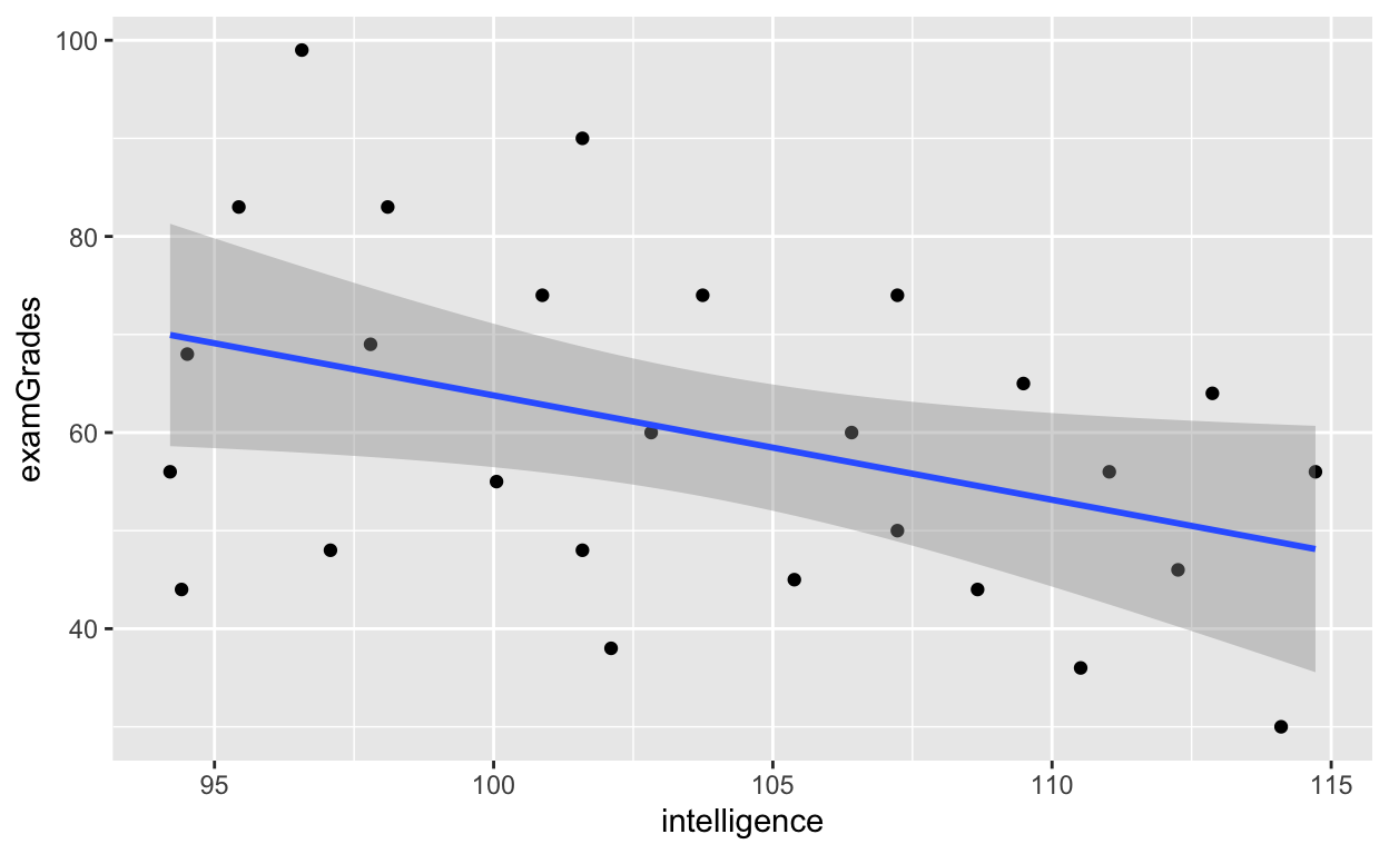
Higher intelligence, worse grades? What's going on? We figure out why later on. And more on ggplot2 package in future tutorials.
Compute summary statistics with summarize() or summarise()
df5 %>% group_by(classroom) %>% # group by classroom summarise(iqMean = mean(intelligence, na.rm = T)) # A tibble: 2 x 2 classroom iqMean <chr> <dbl> 1 a 97.1 2 b 102. df5 %>% group_by(classroom) %>% # group by classroom summarize(iqClassMean = mean(intelligence, na.rm = T), examGradesClassMean = mean(examGrades, na.rm = T)) # A tibble: 2 x 3 classroom iqClassMean examGradesClassMean <chr> <dbl> <dbl> 1 a 97.1 71.4 2 b 102. 55 Same code but with original dataset (dimensions: 40 x 3)
df4 %>% group_by(class) %>% # grouping by class summarise(iqClassMean = mean(iq, na.rm = T), examGradesClassMean = mean(grades, na.rm = T)) # A tibble: 4 x 3 class iqClassMean examGradesClassMean <chr> <dbl> <dbl> 1 a 97.1 71.4 2 b 105. 56.9 3 c 114. 47.9 4 d 122. 38.7 Group by multiple variables/conditions
Randomly generate gender of student for each row of data with sample()
sample(x = c("female", "male"), size = 40, replace = T) # what is this doing [1] "female" "female" "male" "female" "male" "male" "female" "female" [9] "female" "female" "male" "female" "female" "female" "female" "male" [17] "female" "male" "male" "male" "male" "female" "female" "female" [25] "male" "male" "female" "male" "male" "male" "male" "female" [33] "female" "male" "female" "female" "female" "male" "male" "female" df4$gender <- sample(x = c("female", "male"), size = 40, replace = T) # df4 <- mutate(df4, gender = sample(x = c("female", "male"), size = .N, replace = T)) # save output as above Because the gender labels are generated randomly, you'll get different values each time you re-run the code.
df4 iq grades class gender 1: 94.5128 67.9295 a male 2: 95.4359 82.5449 a male 3: 97.7949 69.0833 a female 4: 98.1026 83.3141 a male 5: 96.5641 99.0833 a female 6: 101.5897 89.8526 a male 7: 100.8718 73.6987 a female 8: 97.0769 47.9295 a male 9: 94.2051 55.6218 a female 10: 94.4103 44.4679 a male 11: 103.7436 74.0833 b male 12: 102.8205 59.8526 b female 13: 101.5897 47.9295 b female 14: 105.3846 44.8526 b female 15: 106.4103 60.2372 b female 16: 109.4872 64.8526 b male 17: 107.2308 74.4679 b male 18: 107.2308 49.8526 b male 19: 102.1026 37.9295 b male 20: 100.0513 54.8526 b female 21: 111.0256 56.0064 c male 22: 114.7179 56.0064 c male 23: 112.2564 46.3910 c female 24: 108.6667 43.6987 c female 25: 110.5128 36.3910 c male 26: 114.1026 30.2372 c male 27: 115.0256 39.4679 c female 28: 118.7179 51.0064 c female 29: 112.8718 64.0833 c female 30: 118.0000 55.3000 c male 31: 116.9744 17.5449 d female 32: 121.1795 35.2372 d male 33: 117.6923 29.8526 d female 34: 121.8974 18.3141 d female 35: 123.6410 29.4679 d female 36: 121.3846 53.6987 d female 37: 123.7436 63.6987 d male 38: 124.7692 48.6987 d female 39: 124.8718 38.3141 d female 40: 127.6410 51.7756 d male iq grades class gender Compute mean for each class by gender
df4 %>% group_by(class, gender) %>% # group by class then gender summarise(iqClassMean = mean(iq, na.rm = T), examGradesClassMean = mean(grades, na.rm = T)) # A tibble: 8 x 4 # Groups: class [4] class gender iqClassMean examGradesClassMean <chr> <chr> <dbl> <dbl> 1 a female 97.4 74.4 2 a male 96.9 69.3 3 b female 103. 53.5 4 b male 106. 60.2 5 c female 114. 48.9 6 c male 114. 46.8 7 d female 122. 33.7 8 d male 124. 50.2 More dplyr and tidyverse information
For much more information, see the following sites
- dplyr tutorial/vignette
- official dplyr documentation
- tidyverse
Supercharging your workflow with data.table()
While the syntax of tidyverse and dplyr functions are really easy to understand, they sometimes can be quite long-winded. Using pipes %>% makes your code readable, but is a bit long to read sometimes. Now we'll see how data.table() can shorten all that code while maintaining readability. Also, data.table() is MUCH faster, which is especially useful when dealing with bigger datasets (hundreds of MBs and GBs and even TBs).
If you use fread('filename') to read your dataset into R, then your object is already a data.table. Check it with class(objectName).
df4 iq grades class gender 1: 94.5128 67.9295 a male 2: 95.4359 82.5449 a male 3: 97.7949 69.0833 a female 4: 98.1026 83.3141 a male 5: 96.5641 99.0833 a female 6: 101.5897 89.8526 a male 7: 100.8718 73.6987 a female 8: 97.0769 47.9295 a male 9: 94.2051 55.6218 a female 10: 94.4103 44.4679 a male 11: 103.7436 74.0833 b male 12: 102.8205 59.8526 b female 13: 101.5897 47.9295 b female 14: 105.3846 44.8526 b female 15: 106.4103 60.2372 b female 16: 109.4872 64.8526 b male 17: 107.2308 74.4679 b male 18: 107.2308 49.8526 b male 19: 102.1026 37.9295 b male 20: 100.0513 54.8526 b female 21: 111.0256 56.0064 c male 22: 114.7179 56.0064 c male 23: 112.2564 46.3910 c female 24: 108.6667 43.6987 c female 25: 110.5128 36.3910 c male 26: 114.1026 30.2372 c male 27: 115.0256 39.4679 c female 28: 118.7179 51.0064 c female 29: 112.8718 64.0833 c female 30: 118.0000 55.3000 c male 31: 116.9744 17.5449 d female 32: 121.1795 35.2372 d male 33: 117.6923 29.8526 d female 34: 121.8974 18.3141 d female 35: 123.6410 29.4679 d female 36: 121.3846 53.6987 d female 37: 123.7436 63.6987 d male 38: 124.7692 48.6987 d female 39: 124.8718 38.3141 d female 40: 127.6410 51.7756 d male iq grades class gender class(df4) [1] "data.table" "data.frame" df1 extra group ID 1 0.7 1 1 2 -1.6 1 2 3 -0.2 1 3 4 -1.2 1 4 5 -0.1 1 5 6 3.4 1 6 7 3.7 1 7 8 0.8 1 8 9 0.0 1 9 10 2.0 1 10 11 1.9 2 1 12 0.8 2 2 13 1.1 2 3 14 0.1 2 4 15 -0.1 2 5 16 4.4 2 6 17 5.5 2 7 18 1.6 2 8 19 4.6 2 9 20 3.4 2 10 class(df1) [1] "data.frame" If your object isn't a data.table, you can convert it to one using setDT().
setDT(df1) # setDT() also works (and works without reassignment: no need to use <-) class(df1) # but setDT() doesn't convert your dataset to a tibble class at the same time [1] "data.table" "data.frame" data.table() basics: [i, j, by]
data.table uses a special but extremely concise syntax that only works with objects that have the data.table class associated with them. If you try to use this special syntax on other classes, you'll screw up big time. So check your class or try to convert to or use data.table whenever possible!
data.table[i, j, by]
- i: row (lets you perform row operations like
filter()andslice()) - j: column (lets you perform column operations like
select()andsummarize()andmutate()) - by: group by (equivalent to
group_by())
Filter data.table via i
df4 iq grades class gender 1: 94.5128 67.9295 a male 2: 95.4359 82.5449 a male 3: 97.7949 69.0833 a female 4: 98.1026 83.3141 a male 5: 96.5641 99.0833 a female 6: 101.5897 89.8526 a male 7: 100.8718 73.6987 a female 8: 97.0769 47.9295 a male 9: 94.2051 55.6218 a female 10: 94.4103 44.4679 a male 11: 103.7436 74.0833 b male 12: 102.8205 59.8526 b female 13: 101.5897 47.9295 b female 14: 105.3846 44.8526 b female 15: 106.4103 60.2372 b female 16: 109.4872 64.8526 b male 17: 107.2308 74.4679 b male 18: 107.2308 49.8526 b male 19: 102.1026 37.9295 b male 20: 100.0513 54.8526 b female 21: 111.0256 56.0064 c male 22: 114.7179 56.0064 c male 23: 112.2564 46.3910 c female 24: 108.6667 43.6987 c female 25: 110.5128 36.3910 c male 26: 114.1026 30.2372 c male 27: 115.0256 39.4679 c female 28: 118.7179 51.0064 c female 29: 112.8718 64.0833 c female 30: 118.0000 55.3000 c male 31: 116.9744 17.5449 d female 32: 121.1795 35.2372 d male 33: 117.6923 29.8526 d female 34: 121.8974 18.3141 d female 35: 123.6410 29.4679 d female 36: 121.3846 53.6987 d female 37: 123.7436 63.6987 d male 38: 124.7692 48.6987 d female 39: 124.8718 38.3141 d female 40: 127.6410 51.7756 d male iq grades class gender class(df4) # is it a data.table? [1] "data.table" "data.frame" Different ways to filter via i
df4[i = gender == 'female',] # just female (j, by are NULL) iq grades class gender 1: 97.7949 69.0833 a female 2: 96.5641 99.0833 a female 3: 100.8718 73.6987 a female 4: 94.2051 55.6218 a female 5: 102.8205 59.8526 b female 6: 101.5897 47.9295 b female 7: 105.3846 44.8526 b female 8: 106.4103 60.2372 b female 9: 100.0513 54.8526 b female 10: 112.2564 46.3910 c female 11: 108.6667 43.6987 c female 12: 115.0256 39.4679 c female 13: 118.7179 51.0064 c female 14: 112.8718 64.0833 c female 15: 116.9744 17.5449 d female 16: 117.6923 29.8526 d female 17: 121.8974 18.3141 d female 18: 123.6410 29.4679 d female 19: 121.3846 53.6987 d female 20: 124.7692 48.6987 d female 21: 124.8718 38.3141 d female iq grades class gender df4[gender == 'female',] # i parameter is not required iq grades class gender 1: 97.7949 69.0833 a female 2: 96.5641 99.0833 a female 3: 100.8718 73.6987 a female 4: 94.2051 55.6218 a female 5: 102.8205 59.8526 b female 6: 101.5897 47.9295 b female 7: 105.3846 44.8526 b female 8: 106.4103 60.2372 b female 9: 100.0513 54.8526 b female 10: 112.2564 46.3910 c female 11: 108.6667 43.6987 c female 12: 115.0256 39.4679 c female 13: 118.7179 51.0064 c female 14: 112.8718 64.0833 c female 15: 116.9744 17.5449 d female 16: 117.6923 29.8526 d female 17: 121.8974 18.3141 d female 18: 123.6410 29.4679 d female 19: 121.3846 53.6987 d female 20: 124.7692 48.6987 d female 21: 124.8718 38.3141 d female iq grades class gender df4[i = gender != 'female',] # not female iq grades class gender 1: 94.5128 67.9295 a male 2: 95.4359 82.5449 a male 3: 98.1026 83.3141 a male 4: 101.5897 89.8526 a male 5: 97.0769 47.9295 a male 6: 94.4103 44.4679 a male 7: 103.7436 74.0833 b male 8: 109.4872 64.8526 b male 9: 107.2308 74.4679 b male 10: 107.2308 49.8526 b male 11: 102.1026 37.9295 b male 12: 111.0256 56.0064 c male 13: 114.7179 56.0064 c male 14: 110.5128 36.3910 c male 15: 114.1026 30.2372 c male 16: 118.0000 55.3000 c male 17: 121.1795 35.2372 d male 18: 123.7436 63.6987 d male 19: 127.6410 51.7756 d male df4[gender != 'female',] iq grades class gender 1: 94.5128 67.9295 a male 2: 95.4359 82.5449 a male 3: 98.1026 83.3141 a male 4: 101.5897 89.8526 a male 5: 97.0769 47.9295 a male 6: 94.4103 44.4679 a male 7: 103.7436 74.0833 b male 8: 109.4872 64.8526 b male 9: 107.2308 74.4679 b male 10: 107.2308 49.8526 b male 11: 102.1026 37.9295 b male 12: 111.0256 56.0064 c male 13: 114.7179 56.0064 c male 14: 110.5128 36.3910 c male 15: 114.1026 30.2372 c male 16: 118.0000 55.3000 c male 17: 121.1795 35.2372 d male 18: 123.7436 63.6987 d male 19: 127.6410 51.7756 d male df4[grades > 85,] # rows where grades > 85 iq grades class gender 1: 96.5641 99.0833 a female 2: 101.5897 89.8526 a male # same as filter(df4, grades > 85), but much more concise df4[iq >= 123 & grades < 50] # smart AND failed iq grades class gender 1: 123.6410 29.4679 d female 2: 124.7692 48.6987 d female 3: 124.8718 38.3141 d female df4[iq >= 123 | grades < 50] # smart OR failed iq grades class gender 1: 97.0769 47.9295 a male 2: 94.4103 44.4679 a male 3: 101.5897 47.9295 b female 4: 105.3846 44.8526 b female 5: 107.2308 49.8526 b male 6: 102.1026 37.9295 b male 7: 112.2564 46.3910 c female 8: 108.6667 43.6987 c female 9: 110.5128 36.3910 c male 10: 114.1026 30.2372 c male 11: 115.0256 39.4679 c female 12: 116.9744 17.5449 d female 13: 121.1795 35.2372 d male 14: 117.6923 29.8526 d female 15: 121.8974 18.3141 d female 16: 123.6410 29.4679 d female 17: 123.7436 63.6987 d male 18: 124.7692 48.6987 d female 19: 124.8718 38.3141 d female 20: 127.6410 51.7756 d male Slice (select rows) with indices via i
df4[1:3] # rows 1 to 3 iq grades class gender 1: 94.5128 67.9295 a male 2: 95.4359 82.5449 a male 3: 97.7949 69.0833 a female df4[35:.N] # rows 35 to last row iq grades class gender 1: 123.6410 29.4679 d female 2: 121.3846 53.6987 d female 3: 123.7436 63.6987 d male 4: 124.7692 48.6987 d female 5: 124.8718 38.3141 d female 6: 127.6410 51.7756 d male .N is a shortcut for the last index. If a dataset has 50 rows, the .N has the value 50.
df4[.N] # last row (.N has the value 40 for our dataset) iq grades class gender 1: 127.641 51.7756 d male df4[40] # don't believe? try it iq grades class gender 1: 127.641 51.7756 d male df4[(.N-3):.N] # last four rows iq grades class gender 1: 123.7436 63.6987 d male 2: 124.7692 48.6987 d female 3: 124.8718 38.3141 d female 4: 127.6410 51.7756 d male df4[(40-3):40] # same iq grades class gender 1: 123.7436 63.6987 d male 2: 124.7692 48.6987 d female 3: 124.8718 38.3141 d female 4: 127.6410 51.7756 d male df4[37:40] # same iq grades class gender 1: 123.7436 63.6987 d male 2: 124.7692 48.6987 d female 3: 124.8718 38.3141 d female 4: 127.6410 51.7756 d male Selecting columns via j
df4[, j = grades] # vector [1] 67.9295 82.5449 69.0833 83.3141 99.0833 89.8526 73.6987 47.9295 55.6218 [10] 44.4679 74.0833 59.8526 47.9295 44.8526 60.2372 64.8526 74.4679 49.8526 [19] 37.9295 54.8526 56.0064 56.0064 46.3910 43.6987 36.3910 30.2372 39.4679 [28] 51.0064 64.0833 55.3000 17.5449 35.2372 29.8526 18.3141 29.4679 53.6987 [37] 63.6987 48.6987 38.3141 51.7756 df4[, grades] # same as above, but note the comma, which indicates j via position (i is before the first comma) [1] 67.9295 82.5449 69.0833 83.3141 99.0833 89.8526 73.6987 47.9295 55.6218 [10] 44.4679 74.0833 59.8526 47.9295 44.8526 60.2372 64.8526 74.4679 49.8526 [19] 37.9295 54.8526 56.0064 56.0064 46.3910 43.6987 36.3910 30.2372 39.4679 [28] 51.0064 64.0833 55.3000 17.5449 35.2372 29.8526 18.3141 29.4679 53.6987 [37] 63.6987 48.6987 38.3141 51.7756 class(df4[, grades]) # not a data.table! [1] "numeric" df4$grades # vector (same as above) [1] 67.9295 82.5449 69.0833 83.3141 99.0833 89.8526 73.6987 47.9295 55.6218 [10] 44.4679 74.0833 59.8526 47.9295 44.8526 60.2372 64.8526 74.4679 49.8526 [19] 37.9295 54.8526 56.0064 56.0064 46.3910 43.6987 36.3910 30.2372 39.4679 [28] 51.0064 64.0833 55.3000 17.5449 35.2372 29.8526 18.3141 29.4679 53.6987 [37] 63.6987 48.6987 38.3141 51.7756 class(df4$grades) # not a data.table! [1] "numeric" How to select columns and keep them as data.table?
df4[, .(grades)] # output looks like a table (tibble + local data table) grades 1: 67.9295 2: 82.5449 3: 69.0833 4: 83.3141 5: 99.0833 6: 89.8526 7: 73.6987 8: 47.9295 9: 55.6218 10: 44.4679 11: 74.0833 12: 59.8526 13: 47.9295 14: 44.8526 15: 60.2372 16: 64.8526 17: 74.4679 18: 49.8526 19: 37.9295 20: 54.8526 21: 56.0064 22: 56.0064 23: 46.3910 24: 43.6987 25: 36.3910 26: 30.2372 27: 39.4679 28: 51.0064 29: 64.0833 30: 55.3000 31: 17.5449 32: 35.2372 33: 29.8526 34: 18.3141 35: 29.4679 36: 53.6987 37: 63.6987 38: 48.6987 39: 38.3141 40: 51.7756 grades class(df4[, .(grades)]) # still a data.table! [1] "data.table" "data.frame" df4[, j = .(grades, gender, iq)] # select multiple columns grades gender iq 1: 67.9295 male 94.5128 2: 82.5449 male 95.4359 3: 69.0833 female 97.7949 4: 83.3141 male 98.1026 5: 99.0833 female 96.5641 6: 89.8526 male 101.5897 7: 73.6987 female 100.8718 8: 47.9295 male 97.0769 9: 55.6218 female 94.2051 10: 44.4679 male 94.4103 11: 74.0833 male 103.7436 12: 59.8526 female 102.8205 13: 47.9295 female 101.5897 14: 44.8526 female 105.3846 15: 60.2372 female 106.4103 16: 64.8526 male 109.4872 17: 74.4679 male 107.2308 18: 49.8526 male 107.2308 19: 37.9295 male 102.1026 20: 54.8526 female 100.0513 21: 56.0064 male 111.0256 22: 56.0064 male 114.7179 23: 46.3910 female 112.2564 24: 43.6987 female 108.6667 25: 36.3910 male 110.5128 26: 30.2372 male 114.1026 27: 39.4679 female 115.0256 28: 51.0064 female 118.7179 29: 64.0833 female 112.8718 30: 55.3000 male 118.0000 31: 17.5449 female 116.9744 32: 35.2372 male 121.1795 33: 29.8526 female 117.6923 34: 18.3141 female 121.8974 35: 29.4679 female 123.6410 36: 53.6987 female 121.3846 37: 63.6987 male 123.7436 38: 48.6987 female 124.7692 39: 38.3141 female 124.8718 40: 51.7756 male 127.6410 grades gender iq df4[, .(grades,gender, iq)] # same as above and we often omit j = grades gender iq 1: 67.9295 male 94.5128 2: 82.5449 male 95.4359 3: 69.0833 female 97.7949 4: 83.3141 male 98.1026 5: 99.0833 female 96.5641 6: 89.8526 male 101.5897 7: 73.6987 female 100.8718 8: 47.9295 male 97.0769 9: 55.6218 female 94.2051 10: 44.4679 male 94.4103 11: 74.0833 male 103.7436 12: 59.8526 female 102.8205 13: 47.9295 female 101.5897 14: 44.8526 female 105.3846 15: 60.2372 female 106.4103 16: 64.8526 male 109.4872 17: 74.4679 male 107.2308 18: 49.8526 male 107.2308 19: 37.9295 male 102.1026 20: 54.8526 female 100.0513 21: 56.0064 male 111.0256 22: 56.0064 male 114.7179 23: 46.3910 female 112.2564 24: 43.6987 female 108.6667 25: 36.3910 male 110.5128 26: 30.2372 male 114.1026 27: 39.4679 female 115.0256 28: 51.0064 female 118.7179 29: 64.0833 female 112.8718 30: 55.3000 male 118.0000 31: 17.5449 female 116.9744 32: 35.2372 male 121.1795 33: 29.8526 female 117.6923 34: 18.3141 female 121.8974 35: 29.4679 female 123.6410 36: 53.6987 female 121.3846 37: 63.6987 male 123.7436 38: 48.6987 female 124.7692 39: 38.3141 female 124.8718 40: 51.7756 male 127.6410 grades gender iq # select(df4, grades, gender, iq) # same as above but with select() df4[, grades:gender] # select grades to gender grades class gender 1: 67.9295 a male 2: 82.5449 a male 3: 69.0833 a female 4: 83.3141 a male 5: 99.0833 a female 6: 89.8526 a male 7: 73.6987 a female 8: 47.9295 a male 9: 55.6218 a female 10: 44.4679 a male 11: 74.0833 b male 12: 59.8526 b female 13: 47.9295 b female 14: 44.8526 b female 15: 60.2372 b female 16: 64.8526 b male 17: 74.4679 b male 18: 49.8526 b male 19: 37.9295 b male 20: 54.8526 b female 21: 56.0064 c male 22: 56.0064 c male 23: 46.3910 c female 24: 43.6987 c female 25: 36.3910 c male 26: 30.2372 c male 27: 39.4679 c female 28: 51.0064 c female 29: 64.0833 c female 30: 55.3000 c male 31: 17.5449 d female 32: 35.2372 d male 33: 29.8526 d female 34: 18.3141 d female 35: 29.4679 d female 36: 53.6987 d female 37: 63.6987 d male 38: 48.6987 d female 39: 38.3141 d female 40: 51.7756 d male grades class gender # select(df4, grades:gender) # same as above but with select() # df4[, .(grades:gender)] # this version doesn't work at the moment df4[, c(2, 3, 4)] # via column index/number grades class gender 1: 67.9295 a male 2: 82.5449 a male 3: 69.0833 a female 4: 83.3141 a male 5: 99.0833 a female 6: 89.8526 a male 7: 73.6987 a female 8: 47.9295 a male 9: 55.6218 a female 10: 44.4679 a male 11: 74.0833 b male 12: 59.8526 b female 13: 47.9295 b female 14: 44.8526 b female 15: 60.2372 b female 16: 64.8526 b male 17: 74.4679 b male 18: 49.8526 b male 19: 37.9295 b male 20: 54.8526 b female 21: 56.0064 c male 22: 56.0064 c male 23: 46.3910 c female 24: 43.6987 c female 25: 36.3910 c male 26: 30.2372 c male 27: 39.4679 c female 28: 51.0064 c female 29: 64.0833 c female 30: 55.3000 c male 31: 17.5449 d female 32: 35.2372 d male 33: 29.8526 d female 34: 18.3141 d female 35: 29.4679 d female 36: 53.6987 d female 37: 63.6987 d male 38: 48.6987 d female 39: 38.3141 d female 40: 51.7756 d male grades class gender df4[, -c(2, 3, 4)] # via column index/number (minus/not columns 1, 3, 4) iq 1: 94.5128 2: 95.4359 3: 97.7949 4: 98.1026 5: 96.5641 6: 101.5897 7: 100.8718 8: 97.0769 9: 94.2051 10: 94.4103 11: 103.7436 12: 102.8205 13: 101.5897 14: 105.3846 15: 106.4103 16: 109.4872 17: 107.2308 18: 107.2308 19: 102.1026 20: 100.0513 21: 111.0256 22: 114.7179 23: 112.2564 24: 108.6667 25: 110.5128 26: 114.1026 27: 115.0256 28: 118.7179 29: 112.8718 30: 118.0000 31: 116.9744 32: 121.1795 33: 117.6923 34: 121.8974 35: 123.6410 36: 121.3846 37: 123.7436 38: 124.7692 39: 124.8718 40: 127.6410 iq df4[, 1:3] # via column index/number (1 to 3) iq grades class 1: 94.5128 67.9295 a 2: 95.4359 82.5449 a 3: 97.7949 69.0833 a 4: 98.1026 83.3141 a 5: 96.5641 99.0833 a 6: 101.5897 89.8526 a 7: 100.8718 73.6987 a 8: 97.0769 47.9295 a 9: 94.2051 55.6218 a 10: 94.4103 44.4679 a 11: 103.7436 74.0833 b 12: 102.8205 59.8526 b 13: 101.5897 47.9295 b 14: 105.3846 44.8526 b 15: 106.4103 60.2372 b 16: 109.4872 64.8526 b 17: 107.2308 74.4679 b 18: 107.2308 49.8526 b 19: 102.1026 37.9295 b 20: 100.0513 54.8526 b 21: 111.0256 56.0064 c 22: 114.7179 56.0064 c 23: 112.2564 46.3910 c 24: 108.6667 43.6987 c 25: 110.5128 36.3910 c 26: 114.1026 30.2372 c 27: 115.0256 39.4679 c 28: 118.7179 51.0064 c 29: 112.8718 64.0833 c 30: 118.0000 55.3000 c 31: 116.9744 17.5449 d 32: 121.1795 35.2372 d 33: 117.6923 29.8526 d 34: 121.8974 18.3141 d 35: 123.6410 29.4679 d 36: 121.3846 53.6987 d 37: 123.7436 63.6987 d 38: 124.7692 48.6987 d 39: 124.8718 38.3141 d 40: 127.6410 51.7756 d iq grades class Other ways to select columns
df4[1:4, "grades"] # rows 1 to 4; column grades grades 1: 67.9295 2: 82.5449 3: 69.0833 4: 83.3141 df4[c(2, 5, 8), c("grades", "iq")] # rows 2, 5, 8; column grades and iq grades iq 1: 82.5449 95.4359 2: 99.0833 96.5641 3: 47.9295 97.0769 Column names are stored in an object
cols <- c("gender", "class") df4[, cols] # doesn't work! Error in `[.data.table`(df4, , cols): j (the 2nd argument inside [...]) is a single symbol but column name 'cols' is not found. Perhaps you intended DT[, ..cols]. This difference to data.frame is deliberate and explained in FAQ 1.1. df4[, ..cols] # works! (special syntax) gender class 1: male a 2: male a 3: female a 4: male a 5: female a 6: male a 7: female a 8: male a 9: female a 10: male a 11: male b 12: female b 13: female b 14: female b 15: female b 16: male b 17: male b 18: male b 19: male b 20: female b 21: male c 22: male c 23: female c 24: female c 25: male c 26: male c 27: female c 28: female c 29: female c 30: male c 31: female d 32: male d 33: female d 34: female d 35: female d 36: female d 37: male d 38: female d 39: female d 40: male d gender class Chaining with data.table ("piping")
df4[1:5, 1:3][grades < 80, ][iq > 95, ] # data.table chaining (or piping) iq grades class 1: 97.7949 69.0833 a df4[1:5, 1:3] %>% filter(grades < 80) %>% filter(iq > 95) # same result as above iq grades class 1: 97.7949 69.0833 a Summarize data via j
# compute grand mean iq and rename variable as iq_grand_mean df4[, j = .(iq_grand_mean = mean(iq, na.rm = T))] iq_grand_mean 1: 109.4077 df4[, .(iq_grand_mean = mean(iq, na.rm = T))] # also works iq_grand_mean 1: 109.4077 # also works, but no renaming and returns a vector (not a data.table!) df4[, mean(iq, na.rm = T)] [1] 109.4077 Compare output with summary()
summary(df4) # check mean iq grades class gender Min. : 94.21 Min. :17.54 Length:40 Length:40 1st Qu.:101.41 1st Qu.:42.64 Class :character Class :character Median :109.08 Median :52.74 Mode :character Mode :character Mean :109.41 Mean :53.69 3rd Qu.:117.77 3rd Qu.:64.28 Max. :127.64 Max. :99.08 What about other statistics and variables? Standard deviation?
df4[, .(iq_grand_mean = mean(iq, na.rm = T), iq_sd = sd(iq, na.rm = T), grades_grand_mean = mean(grades, na.rm = T), grades_sd = sd(grades, na.rm = T))] iq_grand_mean iq_sd grades_grand_mean grades_sd 1: 109.4077 10.05791 53.69067 18.41199 Extra stuff…
# standard way to fit regression models lm(formula = grades ~ iq, data = df4) # y predicted by x (grades predicted by iq) Call: lm(formula = grades ~ iq, data = df4) Coefficients: (Intercept) iq 161.1355 -0.9821 # fit linear regression (lm) inside data.table df4[, lm(formula = grades ~ iq)] Call: lm(formula = grades ~ iq) Coefficients: (Intercept) iq 161.1355 -0.9821 Again, note the negative relationship between iq and grades. We'll explore why in future tutorials.
The point here is to show how powerful j is in data.table. j accepts any function. You can't use this syntax if your object is not a data.table.
df4[, summary(lm(formula = grades ~ iq))] # more extensive output Call: lm(formula = grades ~ iq) Residuals: Min 1Q Median 3Q Max -28.715 -12.841 -0.248 11.661 32.779 Coefficients: Estimate Std. Error t value Pr(>|t|) (Intercept) 161.1355 27.5316 5.853 9.07e-07 *** iq -0.9821 0.2506 -3.919 0.000359 *** --- Signif. codes: 0 '***' 0.001 '**' 0.01 '*' 0.05 '.' 0.1 ' ' 1 Residual standard error: 15.74 on 38 degrees of freedom Multiple R-squared: 0.2878, Adjusted R-squared: 0.2691 F-statistic: 15.36 on 1 and 38 DF, p-value: 0.0003592 # summary(lm(formula = grades ~ iq, data = df4)) # standard way to fit regression models Or use the summaryh() function in the hausekeep package to get APA-formatted results and effect size estimates.
If you don't have my package and want to use it, you'll have to install it from github. Run devtools::install_github("hauselin/hausekeep") in your R console (you might have to install devtools install.packages(devtools) first).
df4[, summaryh(lm(formula = grades ~ iq))] term results 1: (Intercept) b = 161.14, SE = 27.53, t(38) = 5.85, p < .001, r = 0.69 2: iq b = −0.98, SE = 0.25, t(38) = −3.92, p < .001, r = 0.54 # summaryh(lm(formula = grades ~ iq, data = df4)) # standard way to fit regression models Compute summary statistics and apply functions to j by groups
What if we want the mean iq and grades for each class? Here is where data.table is much more concise than dplyr and tidyverse.
data.table syntax
df4[, .(iqMean = mean(iq, na.rm = T)), by = class] class iqMean 1: a 97.05641 2: b 104.60514 3: c 113.58973 4: d 122.37948 # omitting by also works, by not recommended because it makes your code very hard to read df4[, .(iqMean = mean(iq, na.rm = T)), class] # not recommended class iqMean 1: a 97.05641 2: b 104.60514 3: c 113.58973 4: d 122.37948 dplyr syntax
df4 %>% group_by(class) %>% summarize(iqMean = mean(iq, na.rm = T)) # A tibble: 4 x 2 class iqMean <chr> <dbl> 1 a 97.1 2 b 105. 3 c 114. 4 d 122. Summarize by class and gender
df4[, .(iqMean = mean(iq, na.rm = T)), by = .(class, gender)] class gender iqMean 1: a male 96.85470 2: a female 97.35898 3: b male 105.95900 4: b female 103.25128 5: c male 113.67178 6: c female 113.50768 7: d female 121.60439 8: d male 124.18803 df4[, .(iqMean = mean(iq, na.rm = T)), keyby = .(gender, class)] # summarize and sort/arrange by class then gender gender class iqMean 1: female a 97.35898 2: female b 103.25128 3: female c 113.50768 4: female d 121.60439 5: male a 96.85470 6: male b 105.95900 7: male c 113.67178 8: male d 124.18803 Summarize by booleans
df4[, .(iqMean = mean(iq, na.rm = T)), by = .(gender == "male")] gender iqMean 1: TRUE 107.9919 2: FALSE 110.6886 df4[, .(iqMean = mean(iq, na.rm = T)), by = .(gender == "male", class == "a")] gender class iqMean 1: TRUE TRUE 96.85470 2: FALSE TRUE 97.35898 3: TRUE FALSE 113.13215 4: FALSE FALSE 113.82503 Combining pipes with data.table and ggplot
df4[, .(iqMean = mean(iq, na.rm = T)), .(class, gender)] %>% # compute class/gender mean ggplot(aes(class, iqMean, col = gender)) + # plot mean values geom_point(position = position_dodge(0.5)) # plot points and dodge points to avoid overlapping 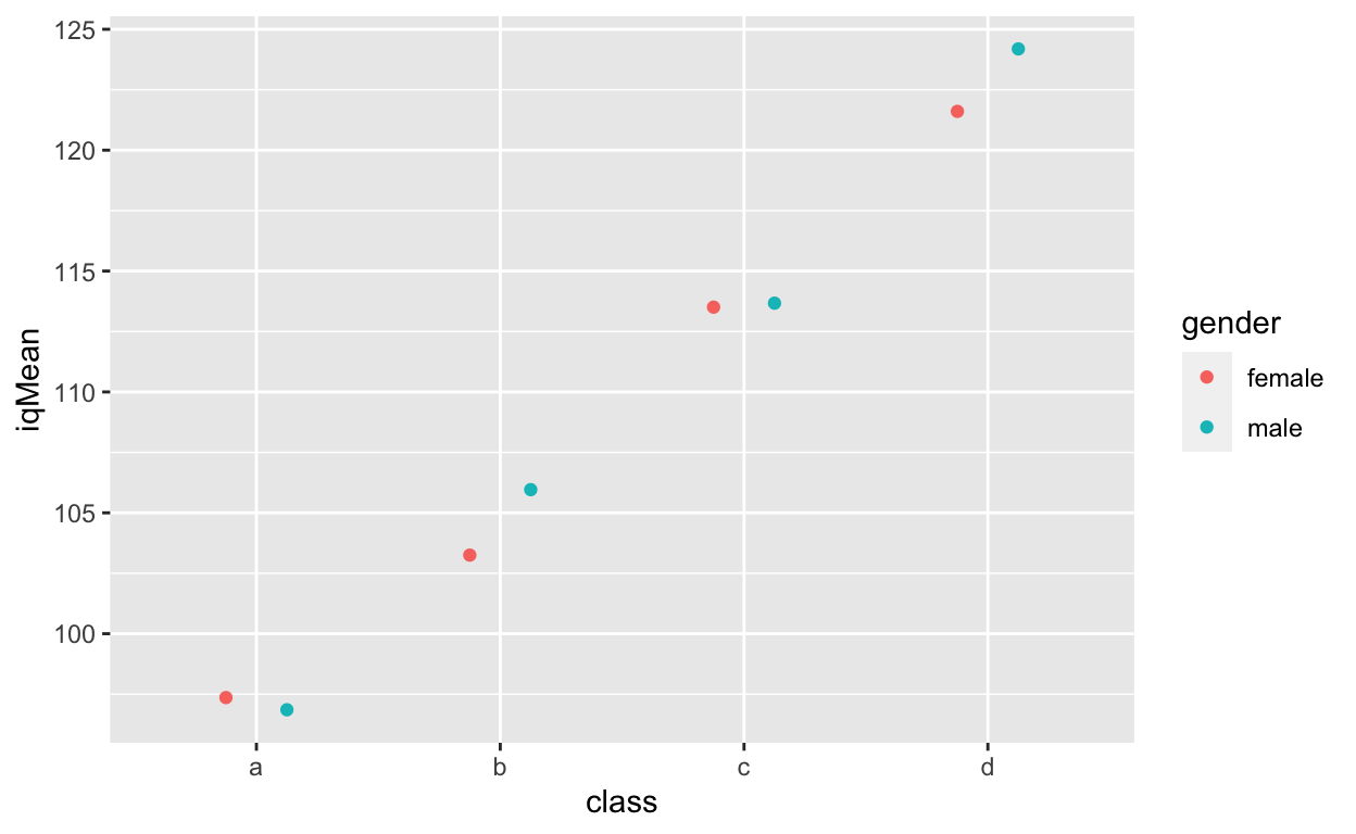
Extra cool stuff again…
- Fit model to entire dataset (grades ~ iq) and use summaryh to summarize model results
df4[, coef(lm(grades ~ iq)), by = class] # get the coefficients for each class class V1 1: a -239.5248083 2: a 3.2030586 3: b -105.9110635 4: b 1.5563490 5: c -29.0664196 6: c 0.6772201 7: d -301.1306213 8: d 2.7765347 df4[, summaryh(lm(grades ~ iq))] term results 1: (Intercept) b = 161.14, SE = 27.53, t(38) = 5.85, p < .001, r = 0.69 2: iq b = −0.98, SE = 0.25, t(38) = −3.92, p < .001, r = 0.54 df4[, summaryh(lm(grades ~ iq)), by = class] # fit model to each class separately class term results 1: a (Intercept) b = −239.52, SE = 210.07, t(8) = −1.14, p = .287, r = 0.37 2: a iq b = 3.20, SE = 2.16, t(8) = 1.48, p = .177, r = 0.46 3: b (Intercept) b = −105.91, SE = 137.69, t(8) = −0.77, p = .464, r = 0.26 4: b iq b = 1.56, SE = 1.32, t(8) = 1.18, p = .271, r = 0.39 5: c (Intercept) b = −29.07, SE = 129.22, t(8) = −0.22, p = .828, r = 0.08 6: c iq b = 0.68, SE = 1.14, t(8) = 0.60, p = .568, r = 0.21 7: d (Intercept) b = −301.13, SE = 165.25, t(8) = −1.82, p = .106, r = 0.54 8: d iq b = 2.78, SE = 1.35, t(8) = 2.06, p = .074, r = 0.59 What we fit just one model to all the data (all 40 rows), what's the relationship between iq and grades? Positive or negative?
And what happens when we fit the model to each class separately, what's the relationship between iq and grades? Positive or negative? We'll explore these relationships in depth in future tutorials.
Creating new variables/columns and reassigning in data.tables with :=
df4[, class := toupper(class)] # convert to upper case head(df4) # print the first few rows of df4 iq grades class gender 1: 94.5128 67.9295 A male 2: 95.4359 82.5449 A male 3: 97.7949 69.0833 A female 4: 98.1026 83.3141 A male 5: 96.5641 99.0833 A female 6: 101.5897 89.8526 A male df4[, class := tolower(class)] # convert to lower case head(df4) iq grades class gender 1: 94.5128 67.9295 a male 2: 95.4359 82.5449 a male 3: 97.7949 69.0833 a female 4: 98.1026 83.3141 a male 5: 96.5641 99.0833 a female 6: 101.5897 89.8526 a male df4[, sex := gender] # make a copy of column # same as df4$sex <- df4$gender head(df4) iq grades class gender sex 1: 94.5128 67.9295 a male male 2: 95.4359 82.5449 a male male 3: 97.7949 69.0833 a female female 4: 98.1026 83.3141 a male male 5: 96.5641 99.0833 a female female 6: 101.5897 89.8526 a male male df4[, sex := substr(sex, 1, 1)] # take only first character # same as df4$sex <- substr(df4$sex, 1, 1) head(df4) iq grades class gender sex 1: 94.5128 67.9295 a male m 2: 95.4359 82.5449 a male m 3: 97.7949 69.0833 a female f 4: 98.1026 83.3141 a male m 5: 96.5641 99.0833 a female f 6: 101.5897 89.8526 a male m df4[, iqCopy := iq] head(df4) iq grades class gender sex iqCopy 1: 94.5128 67.9295 a male m 94.5128 2: 95.4359 82.5449 a male m 95.4359 3: 97.7949 69.0833 a female f 97.7949 4: 98.1026 83.3141 a male m 98.1026 5: 96.5641 99.0833 a female f 96.5641 6: 101.5897 89.8526 a male m 101.5897 df4[iqCopy < 100, iqCopy := NA] # convert values less than 100 to NA head(df4) iq grades class gender sex iqCopy 1: 94.5128 67.9295 a male m NA 2: 95.4359 82.5449 a male m NA 3: 97.7949 69.0833 a female f NA 4: 98.1026 83.3141 a male m NA 5: 96.5641 99.0833 a female f NA 6: 101.5897 89.8526 a male m 101.5897 df4[is.na(iqCopy)] # filter via i (show only rows where iqCopy is NA) iq grades class gender sex iqCopy 1: 94.5128 67.9295 a male m NA 2: 95.4359 82.5449 a male m NA 3: 97.7949 69.0833 a female f NA 4: 98.1026 83.3141 a male m NA 5: 96.5641 99.0833 a female f NA 6: 97.0769 47.9295 a male m NA 7: 94.2051 55.6218 a female f NA 8: 94.4103 44.4679 a male m NA # same as filter(df4, is.na(iqCopy)) df4[iqCopy == NA] # DOESN'T WORK!!! use is.na() Remove a column by assigning a NULL to that column
df4[, iqCopy := NULL] # same as df4$iqCopy <- NULL glimpse(df4) Rows: 40 Columns: 5 $ iq <dbl> 94.5128, 95.4359, 97.7949, 98.1026, 96.5641, 101.5897, 100.871… $ grades <dbl> 67.9295, 82.5449, 69.0833, 83.3141, 99.0833, 89.8526, 73.6987,… $ class <chr> "a", "a", "a", "a", "a", "a", "a", "a", "a", "a", "b", "b", "b… $ gender <chr> "male", "male", "female", "male", "female", "male", "female", … $ sex <chr> "m", "m", "f", "m", "f", "m", "f", "m", "f", "m", "m", "f", "f… df4[, sex := NULL] glimpse(df4) Rows: 40 Columns: 4 $ iq <dbl> 94.5128, 95.4359, 97.7949, 98.1026, 96.5641, 101.5897, 100.871… $ grades <dbl> 67.9295, 82.5449, 69.0833, 83.3141, 99.0833, 89.8526, 73.6987,… $ class <chr> "a", "a", "a", "a", "a", "a", "a", "a", "a", "a", "b", "b", "b… $ gender <chr> "male", "male", "female", "male", "female", "male", "female", … Renaming with setnames()
You don't need to reassign with <- if you use setnames()! See ?setnames to see how this function works.
setnames(df4, "iq", "intelligence") # setnames(datatable, oldname, newname) # if you rename all variables, you don't need to provide the oldname setnames(df4, c("intelligence", "scores", "classroom", "sex")) More data.table information
For more data.table information and tips and tricks, google for them…
- tutorial/vignette
- official documentation
- my own collection of resources
Support my work
Support my work and become a patron here!
Posted by: brown127.blogspot.com
Source: https://hausetutorials.netlify.app/0002_tidyverse_datatable.html